TEC measurement and inversion theory

---

The electron density in the ionosphere can be estimated using dual-frequency measurements of links traversing the ionosphere. The principle of this is shortly explained here.

TEC measurements

Whenever a radio signal is transmitted between two antennas (for instance between a satellite and a ground station), the velocity of the signal depends on the refractive index n of the medium. If this medium is ionised, n depends on the level of ionisation, which relation can be approximated as follows:

n ≈ 1 −

Ne re c 2 2 π f 2

(1)

where:
N_e is the electron density of the medium (electrons/m³);
r_e is the radius of an electron = 2.81794×10^-15 m;
c is the velocity of light in vacuum = 299792458 m/s;
f is the frequency of the signal (Hz).

The time needed for the signal to cover the distance from transmitter to receiver is found by integrating the velocity along the path, and hence depends on the integrated refractive index n. Because of equation (1), this will depend on the integrated electron density N_e. This integrated electron density along the path is referred to as the Total Electron Content, or 'TEC', expressed in electrons/m³×m = electrons/m².

Still, this doesn't help us enough, because we cannot reliably measure the exact time a signal took to reach the receiver. This is why we make use of the dual-frequency beacons of the GPS satellites.

Equation (1) shows that the refractive index also depends on the frequency f of the signal, and hence the total travel time will be different for the two frequencies. By measuring the phase difference between two signals at two different frequencies which traversed the same medium, their difference in travel time can be determined, which is directly related to TEC. From the above can be derived that the relation between phase difference and TEC is:

TEC =

f 1 re c (f 12/f 22 − 1)

Δ&phi

(2)

where:
f₁ and f₂ are the two frequencies of the signals;
Δ&phi is the difference in phase (in radians) between the two signals, defined as:

Δ&phi =

f 1 f 2

&phi2 − &phi1

(3)

where φ₁ and φ₂ are the phases of the two signals.

Using the L1 and L2 signals of GPS, f₁ = 1575.42 MHz and f₂ = 1227.6 MHz, which makes equation (2):

TEC = 2.88255×1015Δ&phi

(4)

Differential TEC

As is always the case with phase measurements, the measurement of the differential phase Δ&phi becomes ambiguous as soon as it's larger than 2π, because a phase of 2π is equal to a phase of zero.

This problem is solved by calculating the change in time of the phase difference. The phase difference in general changes in time, not only because the ionosphere changes, but also the satellites are moving, and therefore the measured path changes continuously.

The phase difference increment between two samples is much smaller than the phase difference itself, and can therefore be unambiguous is if it can be assumed that it's always smaller than π radians (in absolute value). This assumption can be justified if the sample frequency of the GPS signals measurements is high enough.

Because of this, the useful data from the GPS measurements are derived from increments of Δ&phi, and consist of increments of TEC, or differential TEC, referred to as 'dTEC'.

Inversion

As described above, the GPS measurements only give the differential TEC for every measured path between a satellite and a receiver, not the 3-dimensional electron density N_e. However, N_e can be estimated from this under the assumption that enough simultaneously measured crossing paths are avaliable, as illustrated in the figure below. This is done using an inversion procedure.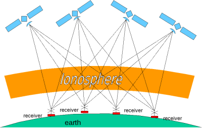

The inversion procedure looks for the electron density distribution as a function of 3D location and time, such that the integrated electron density along the path is equal to the measured TEC, for each path between any satellite and any receiver. Using the differential electron content dTEC, this is expressed as:

∫Ne(x,t)dl − ∫Ne(x,t-dt)dl = dTECl(t)

(5)

where x indicates a 3D location, and dt is the sample time. The integrals are evaluated along the measured path (note that the two paths of the two integrals are generally different!). There is an equation like equation (5) for every measured sample of dTEC.

The solution is searched for a 4-dimensional area which contains the area of the ionosphere where all the relevant measurements are made, and spans a certain period of time. This area is divided in 4D voxels. For each voxel, all equations (5) for all the measurements are linearly combined, with weight factors according to their path length inside the voxel, to result in one equation for this voxel. In the linear combination are also taken along some criteria which minimise the difference between adjacent voxels in horizontal dimensions and time, in order to minimise the temporal end horizontal gradients of electron density. The result of this is one equation for each voxel, which expresses the relation of the electron density of that voxel with that of all other voxels and with the measured values.

Next, the inversion procedure tries to find a solution of 4D electron density which matches this system of equations. It starts from a starting solution (which can be the IRI-ionopshere and a Chapman height profile), and iteratively modifies it, to minimise the error of the system of equations.

Obviously, an exact matching solution will never be found, and the accuracy of the result of the inversion increases with the number of available measurements on crossing paths. Hence, it is beneficial to use as many satellites and receivers as possible.